What is the Standard Risk Measure?
The Standard Risk Measure (SRM) is a guide as to the likely number of negative annual returns expected over any 20 year period. The purpose of the Standard Risk Measure is to provide members with a label to assist in comparing investment options both within and across various superannuation funds.
The Trustee estimates the risk of each investment option based on assumptions about how investment markets are forecast to perform, the likely fluctuation in returns and the relationship between asset classes. These assumptions are not guaranteed.
The SRM will be reviewed annually or in the interim if the Trustee believes there has been a material change to the underlying risk and return assumptions. These risk bands and risk labels are based on the seven categories listed below as provided for in the Standard Risk Measure guidance issued jointly by the Association of Superannuation Funds of Australia Limited and Financial Services Council in July 2011. Set out below is the methodology used by Rest in determining the risks bands and risks labels for its investment options.
| 1 |
Very Low |
Less than 0.5 |
| 2 |
Low |
0.5 to less than 1 |
| 3 |
Low to Medium |
1 to less than 2 |
| 4 |
Medium |
2 to less than 3 |
| 5 |
Medium to High |
3 to less than 4 |
| 6 |
High |
4 to less than 6 |
| 7 |
Very High |
6 or Greater |
| 1 |
| Very Low |
| Less than 0.5 |
| 2 |
| Low |
| 0.5 to less than 1 |
| 3 |
| Low to Medium |
| 1 to less than 2 |
| 4 |
| Medium |
| 2 to less than 3 |
| 5 |
| Medium to High |
| 3 to less than 4 |
| 6 |
| High |
| 4 to less than 6 |
| 7 |
| Very High |
| 6 or Greater |
Rest Methodology
Following is a detailed description of the methodology utilised by Rest to produce expected risk and return calculations for investment portfolios. It should be noted that the underlying methodology is the same as that used by Rest prior to the release of the SRM guidance. There are a few differences to note in how that underlying methodology is applied to ensure that the output is consistent with the SRM guidance. These differences can be summarised as follows:
- The risk output takes the form of the chance of a negative return in x years out of 20.
- The assumptions for returns are based on pre-tax returns not including franking credits as specified within the SRM Guidance Paper issued jointly by The Association of Superannuation Funds of Australia Limited and Financial Services Council in July 2011.
- The expected returns are gross of administration fees but net of investment fees.
- There is allowance in the model to make assumptions with respect to manager outperformance. Generally, Rest will make an assumption that manager outperformance will offset the investment fee and there is scope to add an additional amount if considered appropriate to reflect the expected outperformance of managers.
General Methodology
Rest uses a statistical approach in calculating the return and risk characteristics of a portfolio of assets. This type of approach uses a set of assumptions about the return, volatility and correlations of different assets, combined with an assumption about their distribution, to calculate the portfolio level characteristics.
This statistical approach differs from a simulation approach that may be used by other parties to approach the same problem of expected portfolio return/risk characteristics. A simulation approach may be described as a Monte Carlo approach and uses repeated random sampling to compute the results.
Rest believes this is the most appropriate methodology for the purpose; however every methodology has limitations, and it is important to understand the limitations and implicit assumptions of the approach used.
Assumptions of Rest's Approach
The model Rest uses makes a series of assumptions, including:
- Normal Distribution – Asset class returns are assumed to be normally distributed (i.e. they have a standard bell shaped distribution with a peak at the mean). This assumption is a simplification of reality and assumes zero skewness. This means that returns are symmetrically distributed around the mean. (Negative skewness means there is a substantial probability of a big negative return; positive skewness means that there is a greater-than-normal probability of a big positive return.) The other limitation of a normal distribution is that it has no upper and lower bounds (i.e. it is possible to have a negative return greater than 100% which would not normally be the case without the use of leverage).
- Multi-period rebalancing – The approach considers each individual year as a separate period and in multi-year timeframes, the model assumes that all assets are reweighted back to the starting allocations at the end of each period. There is no re-balancing within the year and the re-weighting is at zero cost.
- Serial correlation (autocorrelation) – Serial correlation is the correlation of a variable with itself over successive time periods, and can be used to determine the expected future state of a variable given its history. The model makes the assumption of zero serial correlation, i.e. that the future return of an asset class is independent of the recent returns of that asset class. (This is counter to theories of momentum or mean reversion).
Calculation of Portfolio Return
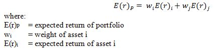
The expected return of the portfolio is calculated as the weighted average of the expected returns of the asset classes which comprise the portfolio. The weights reflect the proportion of the portfolio invested in each asset class.
For example, the expected return of a portfolio of two assets is calculated as:
Calculation of Portfolio Standard Deviation
The portfolio standard deviation is a measure of the risk of the portfolio. The larger the standard deviation, the lower the probability that the actual return will be close to the expected return (i.e. higher risk).
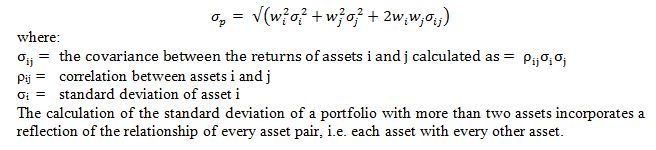
The calculation of the standard deviation of a portfolio includes not only the standard deviations of the component asset classes but also a reflection of how the returns of the asset classes vary against each other (their correlation). This illustrates the benefits of diversification, where the risk of a portfolio of two assets is reduced if the two assets have low or negative correlations to each other.
For example, the standard deviation of a portfolio of two assets is calculated as:
Calculation of Probability of Expected Negative Return for a Portfolio
In order to calculate the probability that the portfolio experiences a negative return in any year, or similarly the probability of negative returns in x out of y years, a further assumption must be made. This assumption is that asset class returns are normally distributed, i.e. they have a standard bell shaped distribution with a peak at the mean.
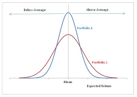
The figure below shows the distribution of expected returns for two different portfolios. The portfolios are both normally distributed and have the same mean (i.e. average expected return) but they have different standard deviations. The standard deviation of portfolio 2 (red line) is greater than that of portfolio 1 (blue line), reflecting a higher risk portfolio, and as a result there are more occasions when the return is significantly greater or smaller than the mean.
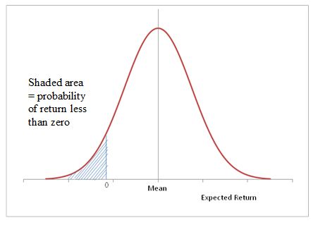
The normal distribution is a distribution of probable outcomes, and as such can be used to help calculate the probability of a negative return for a portfolio. The area under the curve represents the total probability, so that the probability of a negative return is the area under the curve bounded by the limits x = 0 and x = minus infinity, as illustrated by the shaded area in the diagram below: